LLM Pretraining with Continuous Concepts

Paper: arXiv
Authors: Jihoon Tack, Jack Lanchantin, Jane Yu, Andrew Cohen, Ilia Kulikov, Janice Lan, Shibo Hao, Yuandong Tian, Jason Weston, Xian Li
Date of Publication: 12th February 2025

Overview

This paper introduces CoCoMix, a novel LLM pretraining method that leverages continuous concepts for improved performance and interpretability. The core methodology involves using pre-trained sparse auto-encoder (SAE) to decompose hidden states of the LLM being trained into a high-dimensional concept space. Importantly, CoCoMix then identifies the most relevant concepts for predicting the next token using ‘attribution scores’, predicting these selected concepts from the LLM’s residual activations, and finally, integrating these predicted concepts back into the model’s residual stream.

Preliminaries

Let ${\mathbf{h}}_t^{\text{con}}=h_{\text{con}}(\mathbf{x}{)}_t\in {\mathbb{R}}^{d_{\text{con}}}$ be the residual activation of transformer at position $t$.
$d_{con}$ is the dimension of residual stream.

Sparse auto-encoder (SAE)

A sparse auto-encoder projects the residual activations of a transformer at a particular layer into much higher dimensional concept space. When applied to an LLM, the SAE decomposes the hidden state into multiple dimensions, each of which can be viewed as a distinct concept capturing semantically meaningful features. There is a sparsity constraint enforced on the concept space.

Let $E:{\mathbb{R}}^{d_{con}}\to {\mathbb{R}}^C$ be the encoder of SAE, where $C$ is the dimension of concept space $(C>d_{con})$.
Let $D:{\mathbb{R}}^C\to {\mathbb{R}}^{d_{con}}$ be the decoder of SAE.

The reconstruction process of SAE is:

$$C_t^{\text{pre}}=E({\mathbf{h}}_t^{\text{con}})$$

where $c_t^{\text{pre}}\in {\mathbb{R}}^C$ is pre-activation function concept vector in the concept space.

$$c_t=\text{TopK}(c_t^{\text{pre}})$$

where TopK is the activation function (they used TopK in this paper, commonly Jumpy ReLUs are also used amongst many other). TopK zeros out all but top K entries. Intuitively, the remaining K entries each can be viewed as representations of distinct concepts. $c_t\in {\mathbb{R}}^C$

$${\hat{\mathbf{h}}}_t^{\text{con}}=D({\mathbf{c}}_t)$$

where ${\hat{\mathbf{h}}}_t^{\text{con}}\in {\mathbb{R}}^{d_{con}}$ is the reconstructed residual activation.
SAE is trained by minimizing the reconstruction loss: $\Vert {\mathbf{h}}_t^{\text{con}}-{\hat{\mathbf{h}}}_t^{\text{con}}{\Vert }_2^2$. By enforcing TopK sparsity, the SAE isolates the most critical dimensions in $C$ that explain the pretrained model’s features.

Continuous Concept Mixing

Continuous Concept Mixing involves 2 major steps:

1. Using a pre-trained SAE of some other model, architecture involves selecting the most important concepts from the SAE concept space.
2. Residual stream activations of the model being trained are used to predict the selected concepts from the SAE. The predictions are concatenated to the residual activations and the forward pass continues as usual.

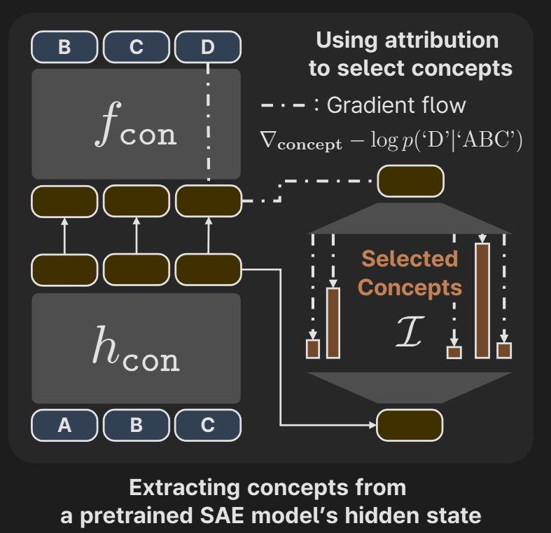
Selecting Important Target Concepts using Attribution Score

While the extracted concepts $C_t$ by SAE represent the core concepts, they may not be useful in predicting the next token. To select the important concepts that help in predicting the next token, authors use attribution.

Let $f_{con}$ represent the entire LLM after the point of $h_{con}$. That is, let the entire LLM be ${\mathcal{M}}_{con}$. Then, ${\mathcal{M}}_{con}=f_{con}\circ h_{con}$.

Authors define attribution score by:

$$a_t=c_t^{\text{pre}}\odot {\nabla }_{c_t}-\log f_{con}(x_{t+1}|D(c_t),h_{<t})$$

Remember that $c_t$ was the concept activation vector after the TopK activation function. ${\nabla }_{c_t}-\log f_{con}(x_{t+1}|D(c_t),h_{<t})$ represents the change in loss (in predicting the next token) with respect to $c_t$. Intuitively, the elements in the gradient vector are large if that particular concept is important, else they are small.
We element-wise multiply the gradient with $c_t^{\text{pre}}$ to obtain the attribution scores. Note that we are multiplying with $c_t^{\text{pre}}$ to also capture the concepts that would have been missed due to TopK. Remember that $a_t,c_t^{\text{pre}},c_t\in {\mathbb{R}}^C$

Next they select the top $K_{attr}$ values of $a_t$. Based on the indices of the top $K_{attr}$ values, authors form $K_{attr}$ one-hot vectors denoted by $\mathcal{I}=\{i_1,\dots ,i_{K_{attr}}\}$, they may not exactly be ‘one-hot’, instead of ‘1’ they were maybe using the $a_t$ score [Disclaimer: Authors don’t explain this part properly in the paper and a lot of details are omitted, I filled in with my best guesses]. These are the targets that the LLM being trained on needs to predict. The

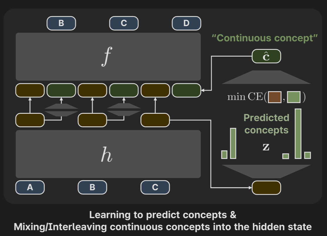
Predicting the selected concepts

Using the residual activations of the LLM, $z_t=M(h_t)\in {\mathbb{R}}^C$ is projected by $M$.

The concept loss is defined as:

$${\mathcal{L}}_{concept}(a_t)=\frac{1}{K_{attr}}\sum _{i\in \mathcal{I}}CE(z_t,i)$$

Authors don’t mention this clearly in the paper, but it looks like a single prediction $z_t$ is made for all the target one-hot vectors in $\mathcal{I}$.

Mixing continuous concepts with token embeddings

The prediction $z_t\in {\mathbb{R}}^C$ that was made previously is projected back to ${\mathbb{R}}^d$:

$${\hat{c}}_t=W\text{TopK}(z_t)+b$$

${\hat{c}}_t\in {\mathbb{R}}^d$ is the ‘continuous concept’. They again used TopK when projecting back in the reverse direction too (from concept space to residual activation space).
Intuitively, we are trying to identify the important concepts and use them for next token prediction. Residual activation was projected to the Concept space, important concepts (that were identified using pre-trained SAE and attribution scores) were predicted, and then it was projected back to the regular activation space. There’s an implicit bias that a given token only uses a few number of concepts, so there’s sparse constraint of TopK.

The ‘continuous concept’ is concatenated with the residual activation. So the residual stream of the model looks like $({\mathbf{h}}_1,{\hat{\mathbf{c}}}_1,\dots ,{\mathbf{h}}_t,{\hat{\mathbf{c}}}_t)$.

This design improves performance and also the predicted concepts $z_t$ can be used to steer the model’s generation process and can be used in alignment.

Training objective

$$\sum _{t=1}^{T-1}-\log f(x_{t+1}|{\mathbf{h}}_{\le t},{\hat{\mathbf{c}}}_{\le t})+\lambda {\mathcal{L}}_{concept}({\mathbf{a}}_t)$$

Next token prediction loss along with the concept prediction loss. $\lambda$ is a hyperparameter.

Authors train 3 models of 69M, 386M and 1.38B sizes. The concept prediction is done at the 4th layer for the 69M model and the 6th layer for the larger 386M and 1.38B models. They used SAE of trained on the 6th layer of 124M parameter GPT-2.

Interpretability and Steerability of CoCoMix

To verify if $z_t$ actually captures concepts, they multiply the vector by constants ranging from -10 to 10. They also do the same in the pre-trained model from which this SAE comes from (i.e. GPT-2 124M).

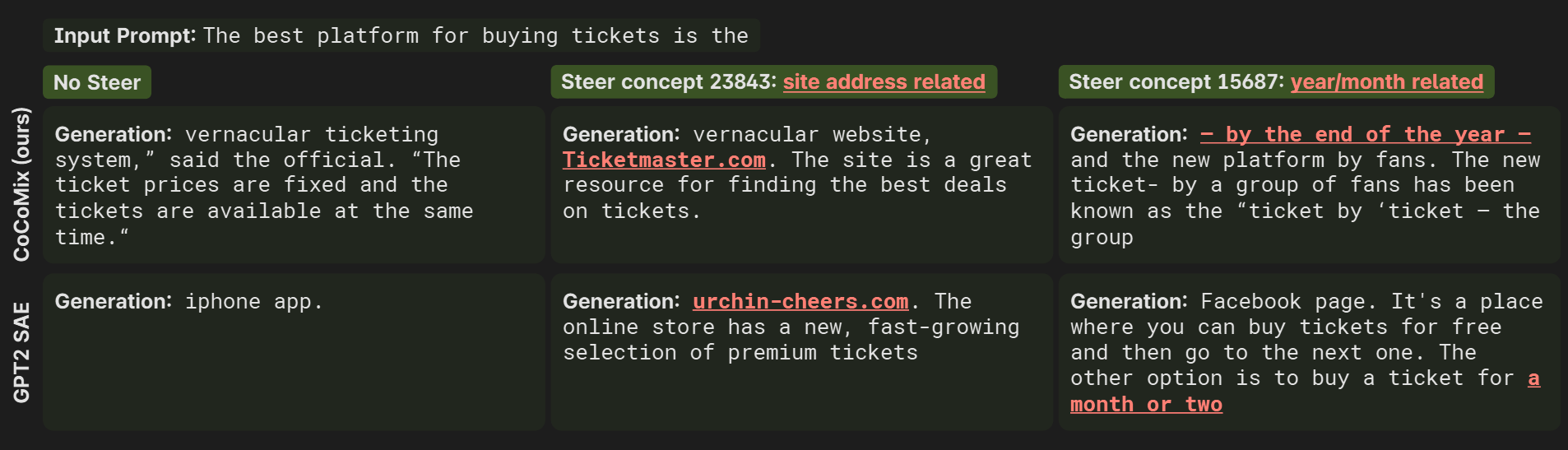
It works!

Results

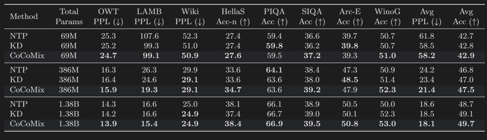
CoCoMix is the architecture of this paper, KD is a model trained on Knowledge Distillation (only with KL divergence between teacher and student as loss), and NTP is a simple decoder only transformer. 124M GPT-2 was used as a teacher-model in all the cases, to keep comparisons fair. CoCoMix slightly beats KD.

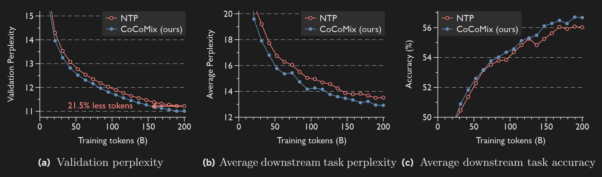
CoCoMix takes 21.5% less tokens when compared to regular decoder-only model to achieve same performance.

There are a lot more experiments done. Check out the paper if you need the details.

Thoughts

A pretty interesting idea. Why distill the knowledge when you can directly ‘suck’ it straight from the concept space.
Implementing this requires so much engineering effort. First we need to obtain a sparse auto encoder of a model whose residual dimension size must be the same as the residual dimension of the model being trained, so that the dimensions match.